Exercise 19.4#
Comparison of RK2, RK4, Gauss–Legendre (s=2), and Radau IIA (s=2)
Overall Process#
Implementation of a generic ExplicitRungeKutta time-stepper
Created ExplicitRungeKutta class in explicitRK.hpp that takes an arbitrary Butcher tableau.
((A,b,c)) with strictly lower triangular (A) (explicit RK).
Definition of specific Butcher tableaus Added setup routines for
RK2 (Heun)
RK4 (classical 4th-order)
Gauss–Legendre IRK (s=2)
Radau IIA IRK (s=2)
Comparison driver
① Implemented Rk_compare.cpp using the ASC-ODE framework and the above time-steppers.
② For each method and each τ, we solve the mass–spring system on \([0,8\pi]\) and write CSV files ex19_4_rk2.csv ex19_4_rk4.csv ex19_4_irk_gauss2.csv``ex19_4_radau2a.csv
Postprocessing / plotting
① plot_RK_methods.py: time evolution and phase plots for each τ.
② plot_RK_errors.py: error vs time, using the exact solution (y(t)=\cos t), (v(t)=-\sin t).
Plots#
Below we summarize the key graphical outputs (only representative examples are shown; full set available in the repository).
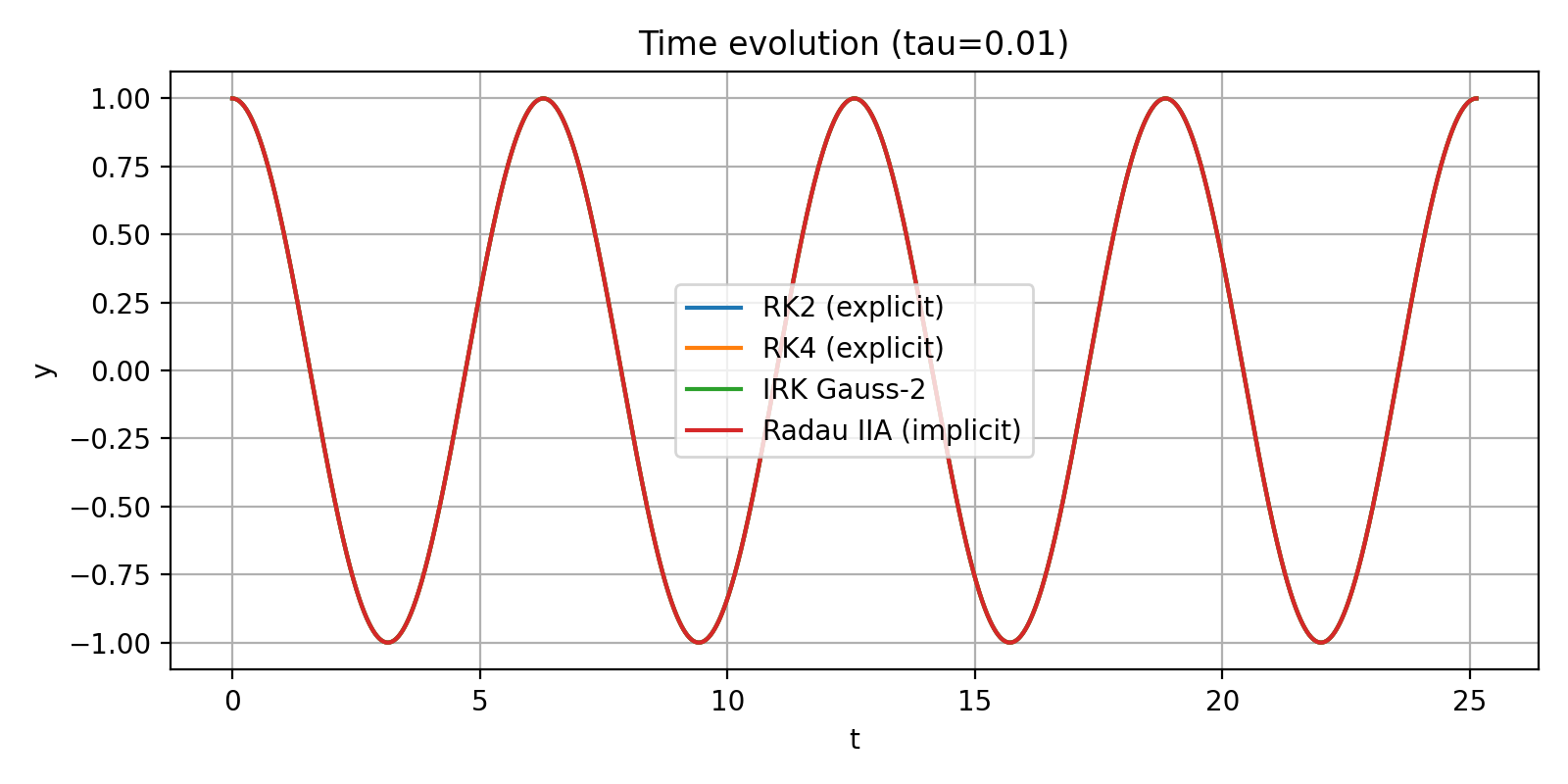
Plot 1 — Time Evolution (τ = 0.01)
All four methods overlap almost perfectly.
Small step size ⇒ high accuracy for all methods; the oscillation keeps correct amplitude and phase.
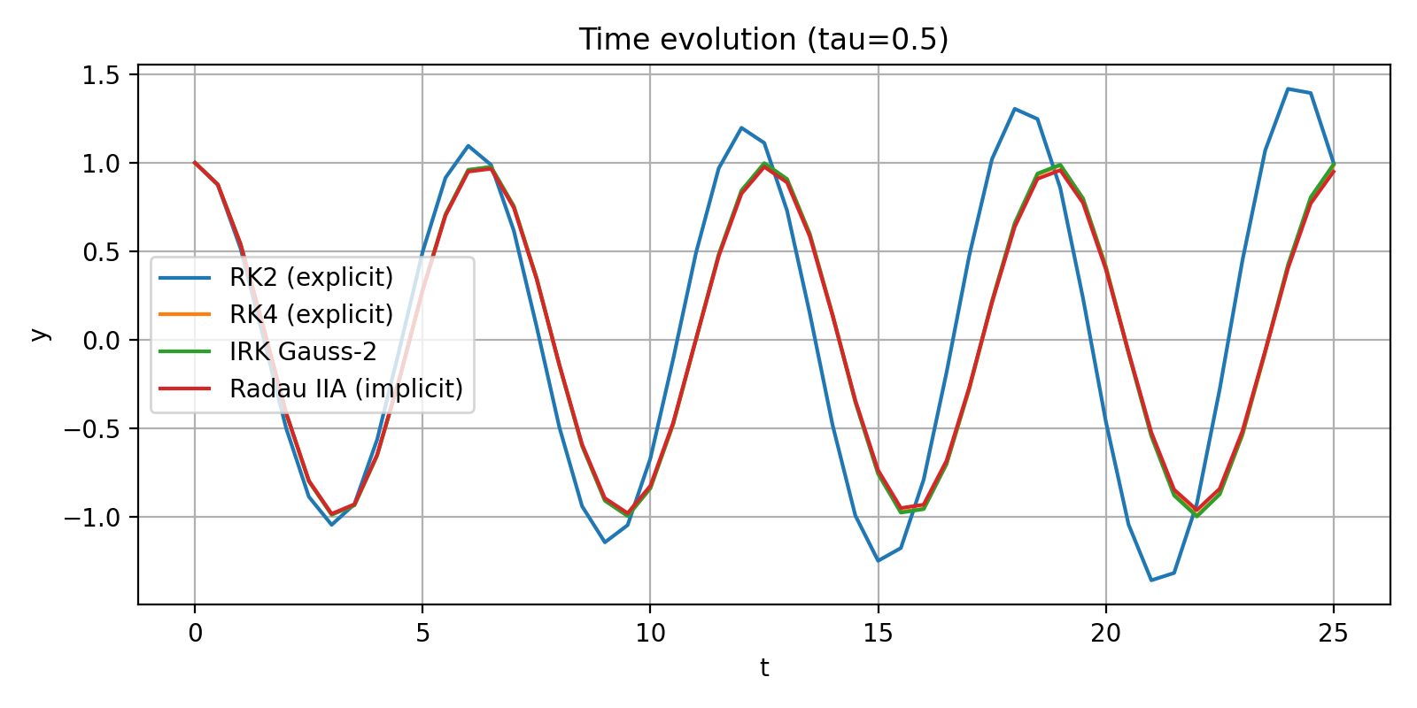
Plot 2 — Time Evolution (τ = 0.5)
Differences become visible:
RK2 starts to lose phase accuracy and amplitude.
RK4 performs better, but a small phase drift appears.
Gauss–Legendre and Radau IIA remain stable and stay close to the true oscillation.
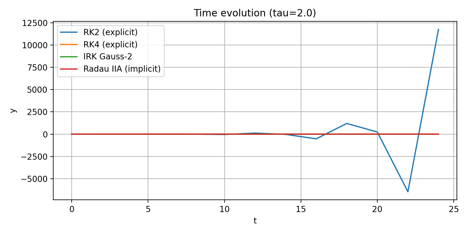
Plot 3 — Time Evolution (τ = 2.0)
RK2 becomes completely unstable and diverges.
RK4 already shows strong distortion.
Radau IIA heavily damps the oscillation (L-stable behavior).
Gauss–Legendre remains bounded but with reduced accuracy due to the very large τ.
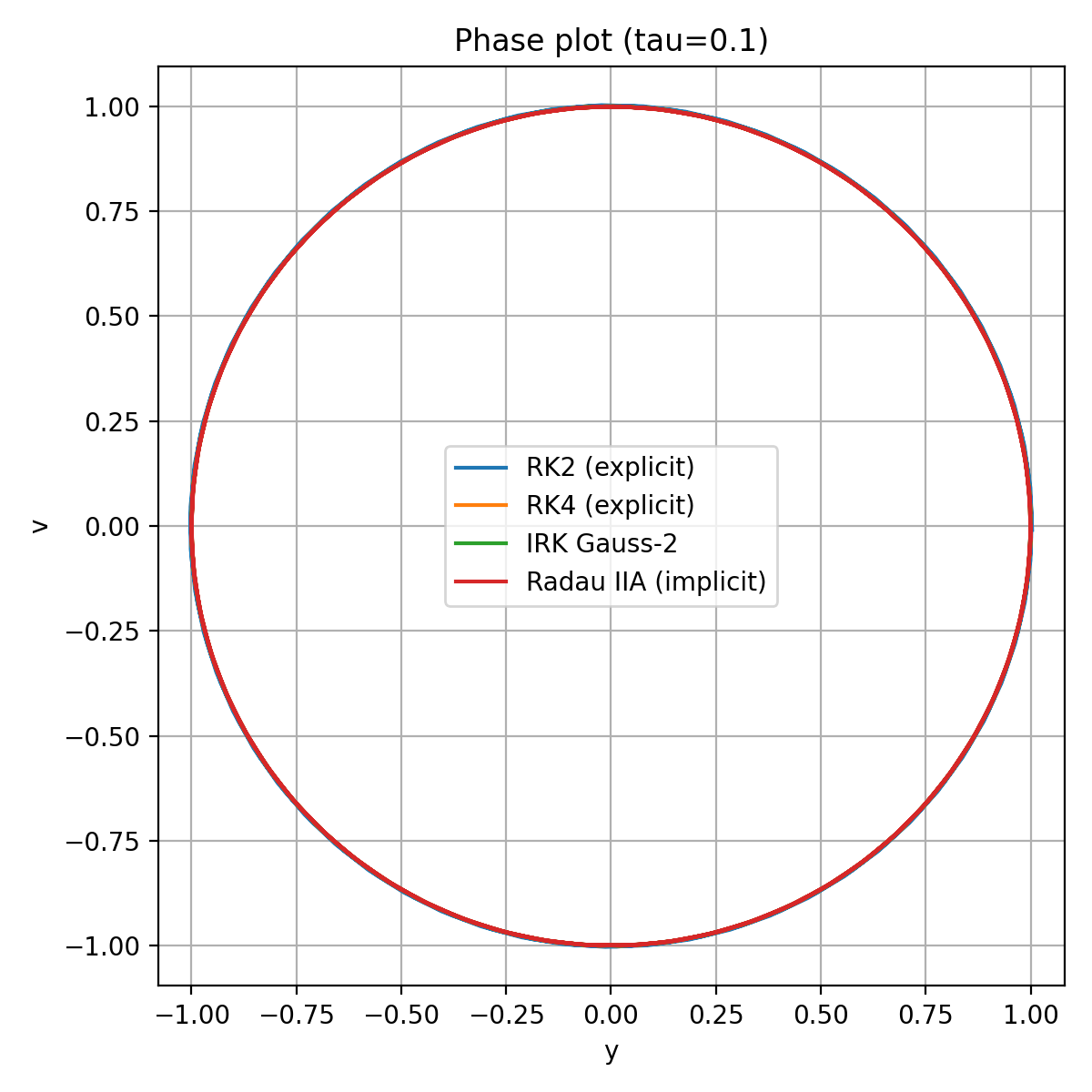
Plot 4 — Phase Portraits (τ = 0.01)
All methods produce nearly perfect circular phase trajectories.
This corresponds to almost energy-conserving behavior at small τ.
Plot 5 — Phase Portraits (τ = 0.5)
RK2 spirals outward ⇒ artificial energy gain.
RK4, Gauss–2, and Radau IIA stay close to the exact circle; trajectories remain bounded.
Plot 6 — Phase Portraits (τ = 2.0)
RK2 spirals dramatically outward (complete loss of stability).
RK4 still oscillatory but clearly distorted.
Gauss–Legendre stays bounded.
Radau IIA spirals inward due to numerical damping (L-stability).
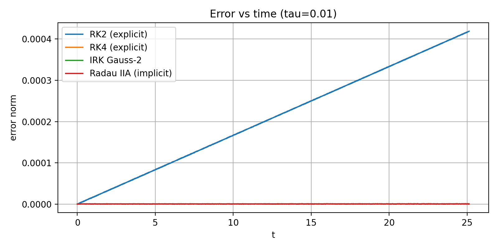
Plot 7 — Error vs Time
For each τ, the error is computed as
$\(
\text{err}(t) = \big\|\,(y_{\text{num}}(t),v_{\text{num}}(t)) - (\cos t,-\sin t)\,\big\|.
\)$
τ = 0.01 and τ = 0.1
RK2: small but steadily growing error.
RK4, Gauss–2, Radau IIA: extremely small errors; curves almost coincide.
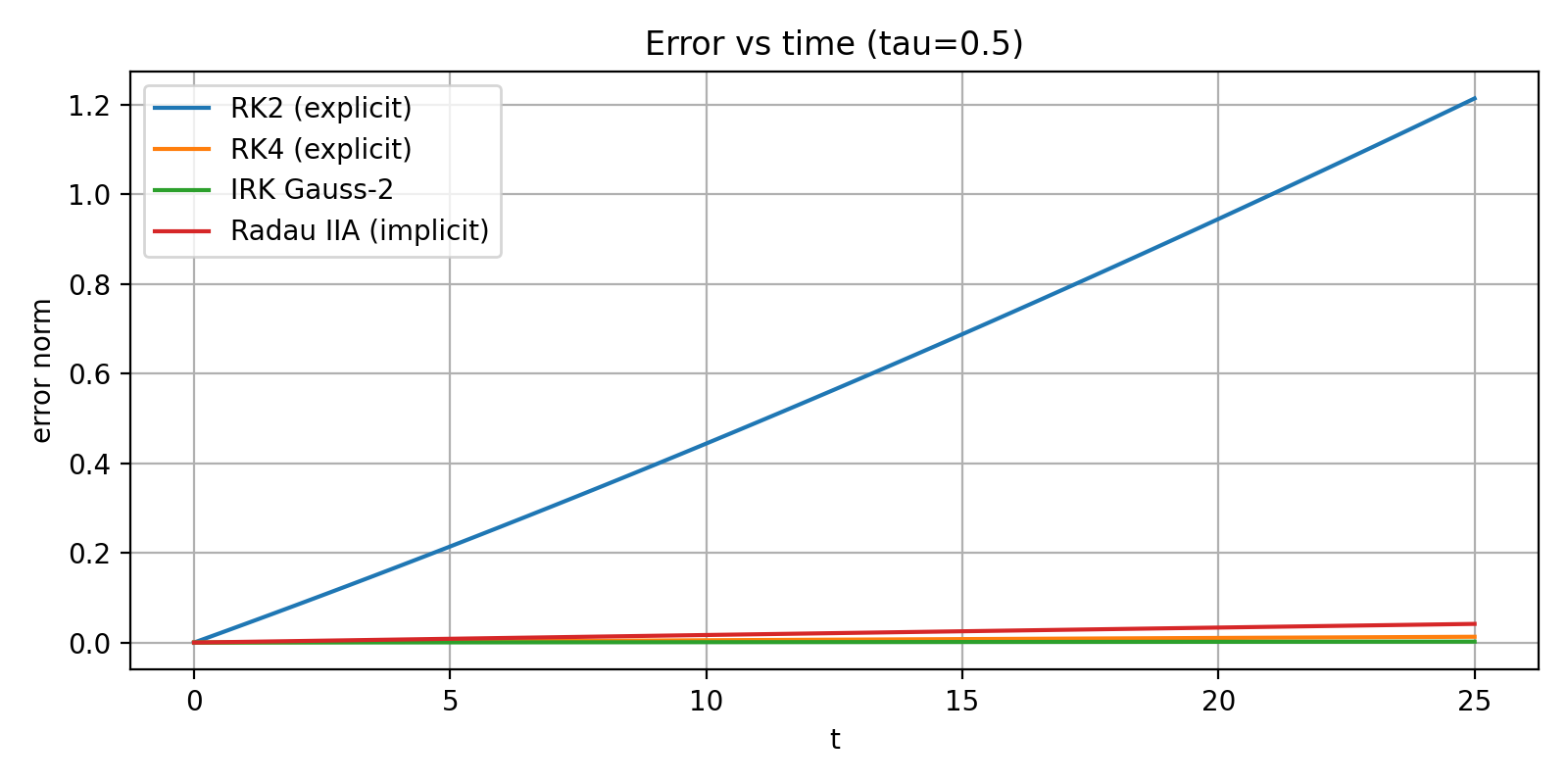
τ = 0.5
RK2: error of order O(1) over the time interval.
RK4: mild growth, still acceptable.
Gauss–2 and Radau IIA: error stays very small and almost bounded.
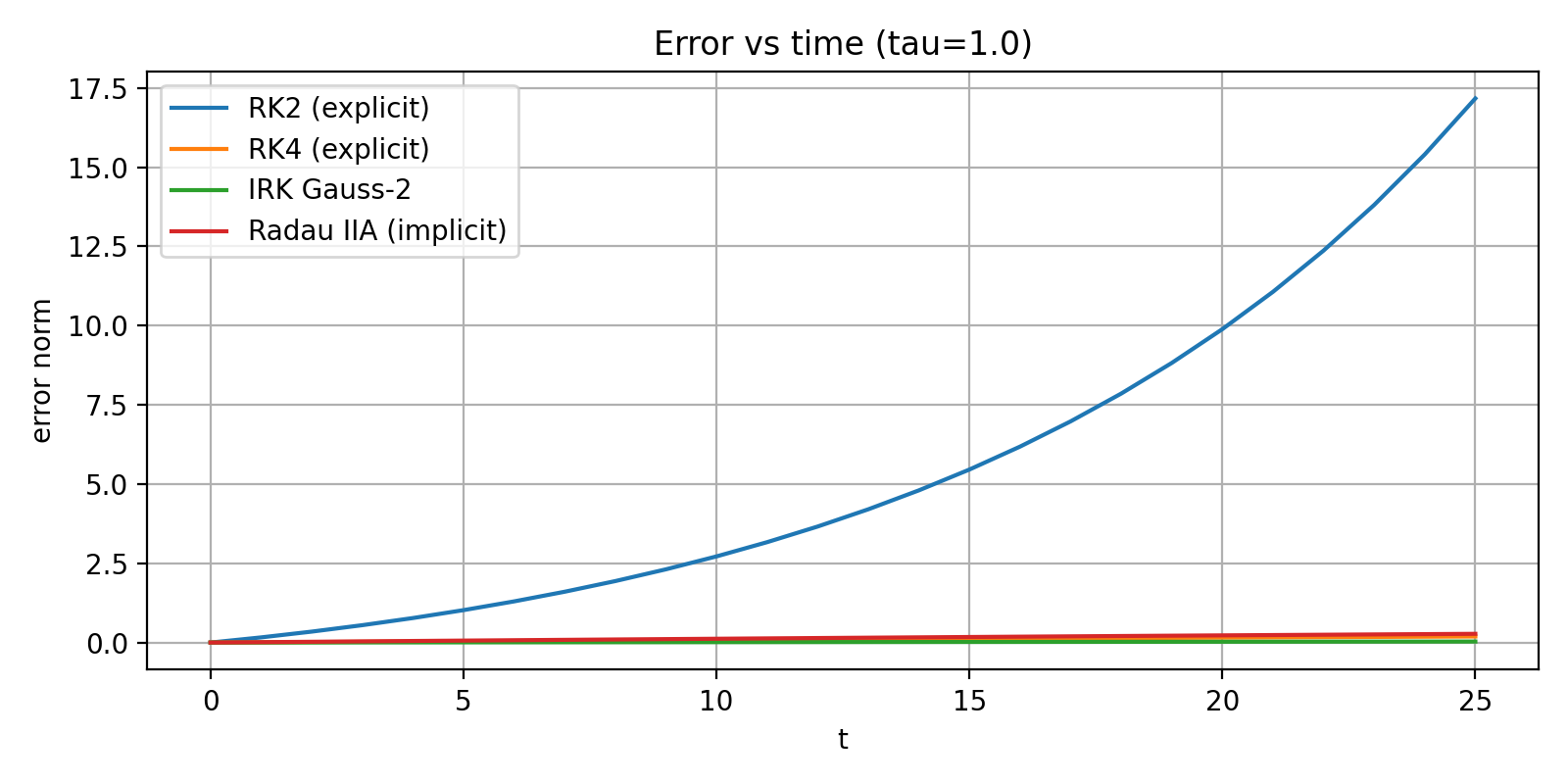
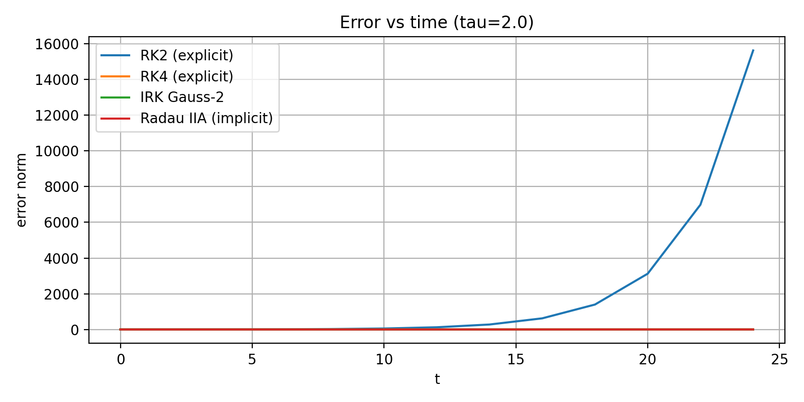
τ = 1.0 and τ = 2.0
RK2: error grows catastrophically (instability).
RK4: significant drift but still bounded.
Gauss–Legendre: stable with moderate error.
Radau IIA: best stability; error remains small even for τ = 2.0.
Conclusions#
ExplicitRungeKutta implementation
The generic
ExplicitRungeKuttatime-stepper successfully handles arbitrary explicit Butcher tableaus with a lower triangular (A).RK2 and RK4 are obtained only by providing their coefficients, confirming that the implementation is method-agnostic and reusable.
RK2 (Explicit Heun)
Second-order accuracy; works well only for small τ.
For τ ≥ 0.5, strong phase and amplitude errors accumulate.
For τ ≥ 1.0, RK2 becomes numerically unstable for the oscillatory system.
RK4 (Classical Explicit)
Much better long-time accuracy than RK2.
Still not A-stable: for very large τ, phase errors become dominant.
Reasonable choice for moderate τ when an explicit scheme is required.
Gauss–Legendre IRK (s=2)
A-stable and symplectic.
Preserves the qualitative structure of the oscillation very well, even for larger τ.
Error remains bounded for all tested step sizes; phase plots stay close to a circle.
Radau IIA IRK (s=2)
L-stable implicit method: damps high-frequency / stiff components.
Extremely robust for large τ; the solution does not blow up.
Shows numerical damping on this pure oscillatory problem, but has the best stability among all tested methods.