Exercise 18.5#
AutoDiff Pendulum
Overall Process#
Adapted the C++ file
ex18_5.cppto simulate the nonlinear pendulum using
with AutoDiff-based Jacobian evaluation.
Generated output trajectory file:
ex18_5.csvCreated Python scripts to plot:
pendulum_time.png— Time evolution of θ(t) and ω(t)pendulum_phase.png— Phase portrait (θ vs ω)
Plots#
Plot 1 – Time Evolution of Pendulum (Explicit Euler)#
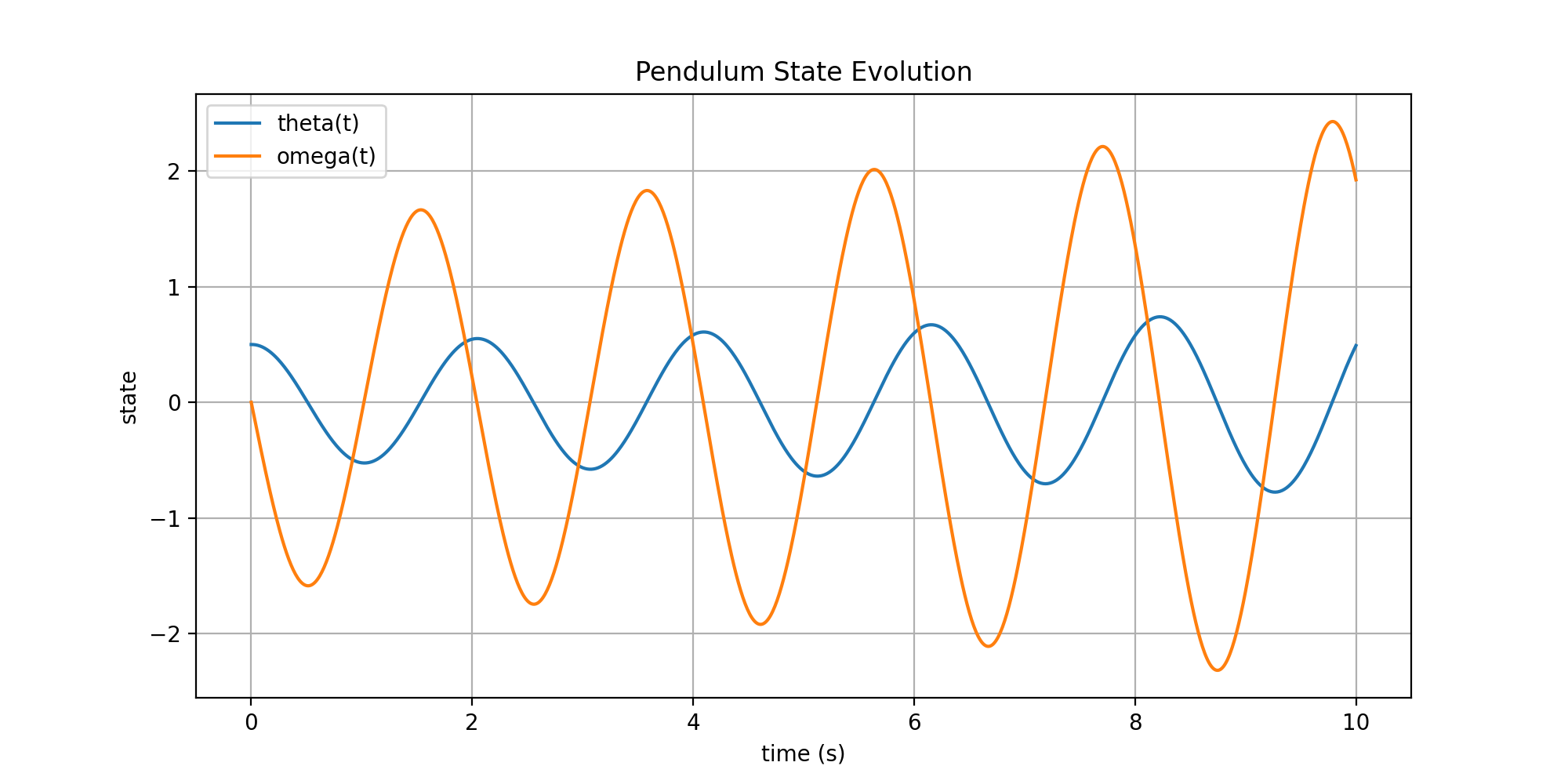
This plot shows the temporal evolution of the pendulum state variables:
θ(t) : angular displacement
ω(t) : angular velocity
Euler integration introduces numerical energy growth over time.
Plot 2 – Phase Plot (Explicit Euler)#
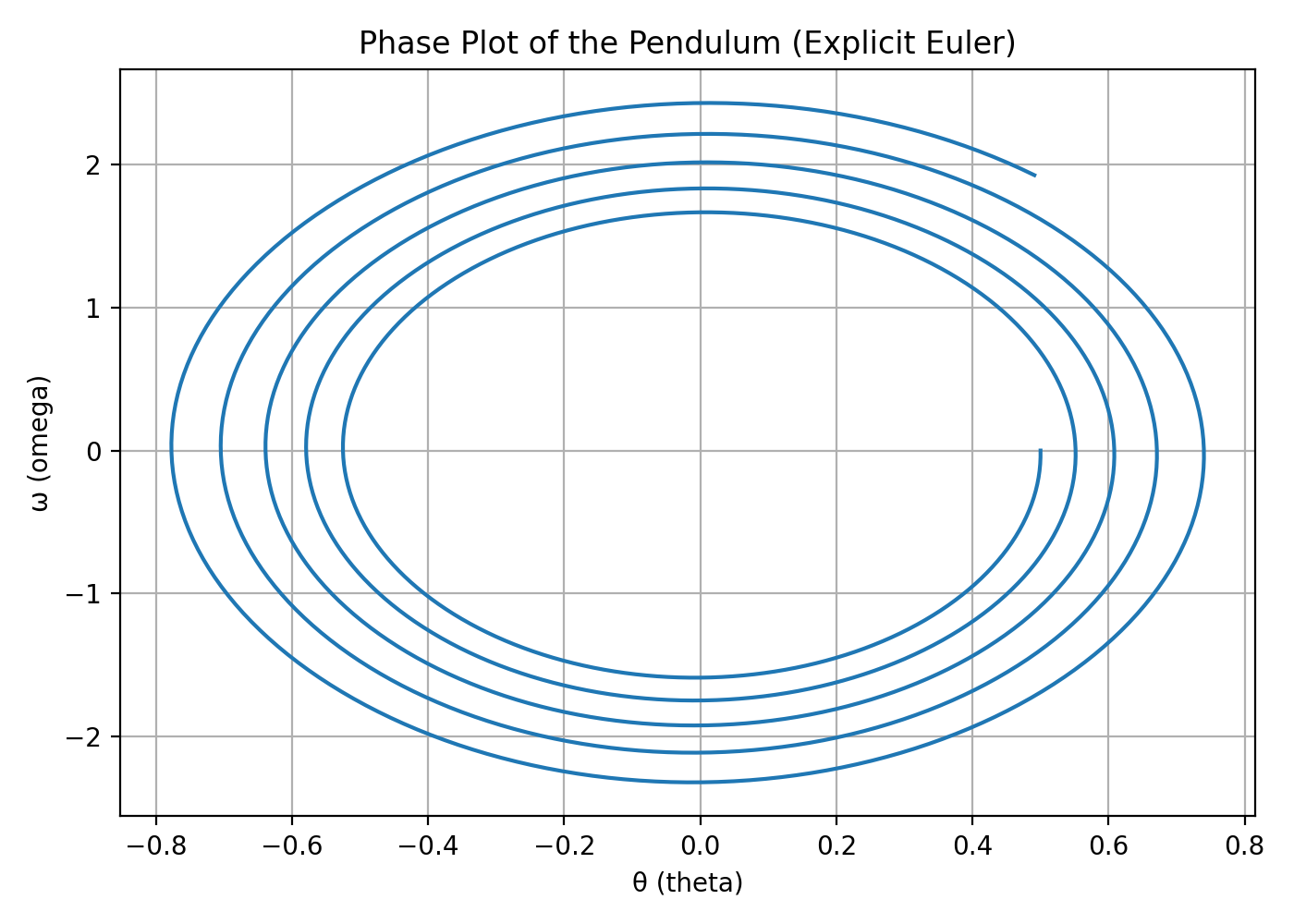
This is the θ–ω phase portrait of the nonlinear pendulum.
A true physical pendulum would trace closed orbits (constant energy), but explicit Euler causes energy to drift.
Conclusion#
The explicit Euler method behaves numerically unstable for oscillatory systems like the pendulum.
The time evolution plot shows that both \( \theta(t) \) and \(\omega(t)\) exhibit increasing amplitude, indicating energy gain.
The phase portrait spirals outward instead of forming closed loops:
This means energy is not conserved numerically.
The trajectory grows unphysically over time.
AutoDiff successfully computes Jacobians for the nonlinear pendulum model.