Exercise 17.4.1#
Q1 : Overall Process#
Adapted Implicit_Euler.cpp to get implicit_euler.csv. Then adapted plotq2.1.py and get graph plot5 and plot6.
Q1 : Plot#
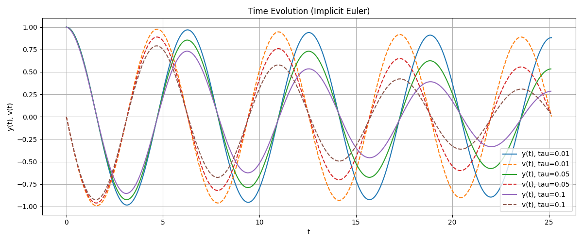
Plot 5 : Time Evolution (implicit euler)#
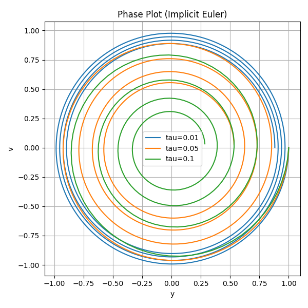
Plot 6 : Phase Plots (implicit euler)#
Q2 : Overall Process#
The general function of Crank-Nicolson method is:
u_{n+1} - u_n - (tau/2)*(f(u_{n+1}) + f(u_n)) = 0
Adapted
Crank_Nicolson.cppto getcrank_nicolson.csv. Then adaptedplotq2.2.pyand get graphplot7andplot8.
Q2 : Plot#
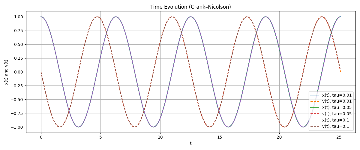
Plot 5 : Time Evolution (Crank-Nicolson)#
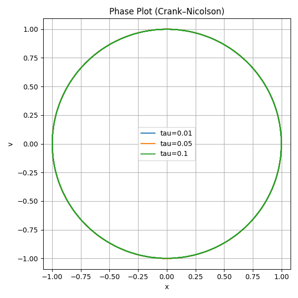
Plot 6 : Phase Plots (Crank-Nicolson)#
Q3 : Comparison of the Four Time-Stepping Methods#
Now we compare 4 methods in previously mentioned:
Explicit Euler
The method is unstable for oscillatory systems.
For moderate or even small time-steps, the numerical orbit in the phase plane spirals outward, corresponding to an artificial gain of energy.
Larger time-steps lead to very rapid divergence.
Improved Euler
Shows second-order accuracy and significantly better behavior.
The phase curves stay close to a circle, even for larger time-steps.
There is still a small drift, but the energy error remains bounded and does not grow dramatically like in Explicit Euler.
Implicit Euler
Always stable, regardless of time-step size.
However, the solution exhibits numerical damping: the phase orbit spirals inward, meaning the method artificially removes energy from the system.
Crank–Nicolson
It is the one given the best results. Always stable, and energy-preserving method for linear oscillatory systems.
The phase plots remain almost perfectly circular for all tested time-steps.
In General:
For oscillatory systems -- the mass–spring model, Crank–Nicolson provides the most physically accurate long-time behavior, while Explicit Euler is the worst method.