Exercise 17.2.2

Q1 : Overall Process

1. Adapted the Explicit_Euler.cpp to get explicit_euler.csv.

2. Adapted the plotq1.py to get performance plot plot1_time_evolution.png and plot2_phase.png.

3. Attention: Add .cpp path into CMakeLists.txt such that we can compile directly.

Q1 : Plot

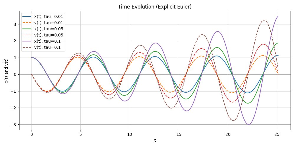
Plot 1 : Time Evolution (explicit euler)

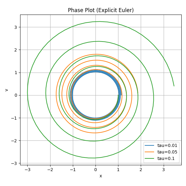
Plot 2 : Phase Plots (explicit euler)

Q1 : Conclusion

• In time evolution plots, both x(t) and v(t) show increasing amplitude, and the growth becomes faster for larger time steps.

• In phase plots clearly illustrate this behavior: instead of forming closed circles (energy conservation), the trajectories spiral outward.

• Overall, explicit Euler is numerically unstable for this oscillatory system, and bigger step sizes make worse.

---

Q2 : Overall Process

Similar with Q1, adapted Improved_Euler.cpp to get improved_euler.csv. Then adapted plotq2.py and get graph plot3 and plot4.

Q2 : Plot

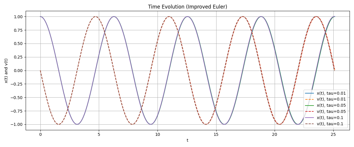
Plot 3 : Time Evolution (improved euler)

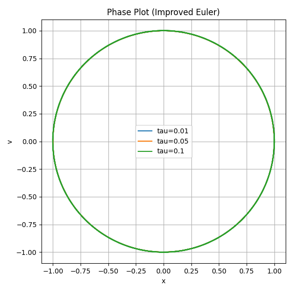
Plot 4 : Phase Plots (improved euler)

Comparison: Explicit Euler Method vs Improved Euler Method

• Obviously, the Improved Euler method shows significantly better stability and accuracy for the mass–spring system.

• For all three time steps, the time-evolution plots indicate that Improved Euler preserves both the amplitude and phase of the oscillation almost perfectly over long times. In contrast, Explicit Euler exhibits clear fluctuation.

• The phase plots further highlight this difference: Improved Euler produces closed circular trajectories that remain nearly identical for all tau, indicating near-conservation of energy. Explicit Euler, however, generates outward-spiraling curves whose radius increases with time, especially for larger tau.